import numpy as np 
import pandas as pd
import torch
import torch.optim as optim
from torch.utils.data import DataLoader
import matplotlib.pyplot as plt
import warnings
warnings.filterwarnings('ignore')
from stengression import GCEN, STEN, MVEN, GraphInfo, SpatioTemporalDataset 
from stengression import compute_adjacency_matrix, prepare_spatial_weights, plot_forecasts, energy_score_loss

1. Prepare the distances and adjacency matrix

# Load the matrix containing Haversine distances for each node and compute the adjacency matrix
distances = pd.read_csv("Belgium_Distance_Matrix.csv")
dist_array = distances.values
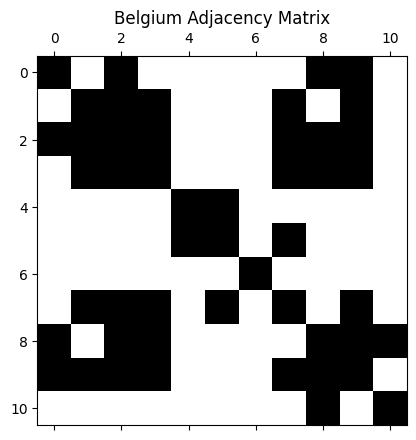
adjacency_matrix = compute_adjacency_matrix(distances.values, sigma2=0.9948808074595779, epsilon=0.07692416606625796, n=40)
np.fill_diagonal(adjacency_matrix, 1)
plt.spy(adjacency_matrix)
plt.title("Belgium Adjacency Matrix")
plt.show()

node_indices, neighbor_indices = np.where(adjacency_matrix == 1)
graph_info = GraphInfo(
    edges=(node_indices.tolist(), neighbor_indices.tolist()),
    num_nodes=adjacency_matrix.shape[0],
)
print(f"Number of nodes: {graph_info.num_nodes}, Number of edges: {len(graph_info.edges[0])}")

Number of nodes: 11, Number of edges: 49

device = torch.device("cuda" if torch.cuda.is_available() else "cpu")
graph_conv_params = {
                "aggregation_type": "mean", # mean, sum, max
                "combination_type": "concat",
                "activation": None
            }
gcn_seed = 21
temporal_seed = 9
print(f'Using device: {device}.')

Using device: cuda.

2. Prepare the training dataset

# Forecast horizon: 30 days
NUM_NODES = 11
IN_FEAT_DIM = 1   # D

P_LAG = 60        # Lag window, input_seq_len
T_PRED = 30        # Prediction horizon, output_seq_len
BATCH_SIZE = 64

alpha, max_spatial_lag = 1,2 
W = 1/(dist_array**alpha)
np.fill_diagonal(W, 0)
row_sums = W.sum(axis=1, keepdims=True)
W = W / row_sums
W = torch.tensor(W)
# W is the initial spatial weights matrix

W_list = prepare_spatial_weights(W, max_lag=max_spatial_lag)

df = pd.read_csv("Belgium_Covid_Nodates.csv", encoding='latin-1')
sts_data = torch.tensor(df.values, dtype=torch.float32)
sts_data=sts_data.view(sts_data.shape[0], sts_data.shape[1], 1) # Converts into T x N x 1
sts_data.to(device)
node_names = df.columns.tolist()

train_tensor = sts_data[:-T_PRED, :, :]
test_ground_truth = sts_data[-T_PRED:, :, :] # The ground truth for the first forecast window is the first T_PRED steps of the test set
test_history = train_tensor[-P_LAG:, :, :] # The history required to make this forecast is the last P_LAG steps of the training set

# Standardize train data
y_train = train_tensor.clone()
mean, std = train_tensor.mean(axis=0), train_tensor.std(axis=0)
train_tensor = ((train_tensor - mean) / std)
test_history = ((test_history - mean) / std) 

# Caution: Do not standardize test_ground_truth, as we want to compare the real forecast values. 
train_dataset = SpatioTemporalDataset(train_tensor, input_seq_len=P_LAG, output_seq_len=T_PRED, multi_horizon=True)
trainloader = DataLoader(train_dataset, batch_size=BATCH_SIZE, shuffle=False)

3. MVEN

3.1 Training the MVEN model

mven = MVEN(in_feat_dim=IN_FEAT_DIM, 
           lstm_hidden_dim=72, lstm_num_layers=3, 
            lstm_dropout=0.09462213176635498, noise_dist="uniform",
           p_lag=P_LAG, t_pred=T_PRED, 
            num_nodes=NUM_NODES, temporal_seed=9).to(device)
optimizer = optim.Adam(mven.parameters(), lr=0.00440078425059993) 

# Run Training
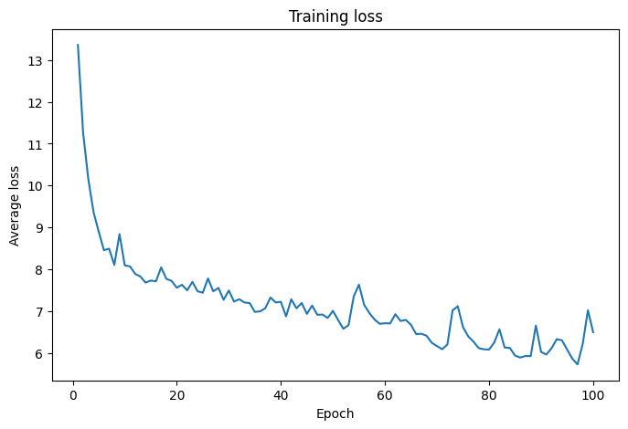
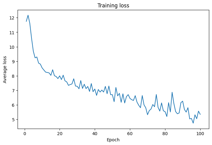
mven.fit(data_loader=trainloader, optimizer=optimizer, loss_fn=energy_score_loss, num_epochs=100, m_samples=2, 
         device=device, monitor=True, visualize=True, verbose=False)

Training: 100%|██████████| 100/100 [00:30<00:00,  3.32epoch/s]

3.2 In-sample Diagnostics

# Getting the un-standardized in-sample predictions
in_sample_preds = mven.predict_in_sample(train_tensor, m_samples = 100, method = "q_step", batch_size = 64, 
                                         device=device, unstandardize=[mean, std])

in_sample_preds.shape

torch.Size([100, 746, 11, 1])

# Evaluation of in-sample predictions
mven.evaluate_in_sample_fit(train_tensor, m_samples = 100, n_repeats = 10,
        method = "q_step", batch_size = 64, point_method="median",
        unstandardize = [mean,std], device = device)

	SMAPE	MAE	RMSE	MASE	RMSSE	Pinball_80	Pinball_95	Rho-0.5	Rho-0.9	CRPS	EC	Winkler
mean	67.11	224.55	565.75	1.15	1.15	111.72	85.06	0.46	0.4	185.68	0.54	4278.32
std	0.11	0.61	2.43	0.00	0.00	0.45	0.60	0.00	0.0	0.29	0.00	32.22

# Getting the residuals
residuals = mven.get_residuals(in_sample_preds, y_train, point_method="median")
residuals.shape

torch.Size([746, 11, 1])

# Plotting the in-sample predictions vs training data and residuals
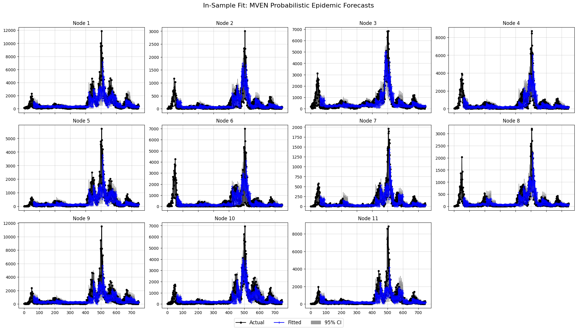
mven.plot_in_sample_fit(
    in_sample_preds=in_sample_preds,
    original_data=y_train, # Ensure ground truth is also in original scale
    plots_per_row=4,
    confidence_level=0.95,
    title="In-Sample Fit: MVEN Probabilistic Epidemic Forecasts"
)

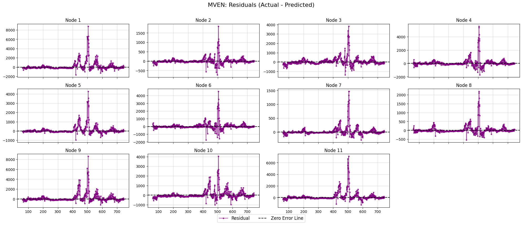
mven.plot_residuals(
    residuals=residuals,
    plots_per_row=4,
    title="MVEN: Residuals (Actual - Predicted)"
)

3.3 Out-of-sample Forecasts and Evaluation

forecast_ensemble = mven.predict(m_samples=100, history=test_history, unstandardize=[mean, std], device=device)
forecast_ensemble.shape

torch.Size([100, 30, 11, 1])

metrics = mven.evaluate_forecasts(m_samples=100, n_repeats=50, 
                              history=test_history, y_true=test_ground_truth, y_train=y_train, 
                              unstandardize=[mean, std])
metrics

	SMAPE	MAE	RMSE	MASE	RMSSE	Pinball_80	Pinball_95	Rho-0.5	Rho-0.9	CRPS	EC	Winkler
mean	66.41	95.81	127.96	0.49	0.26	35.56	15.81	0.54	0.27	72.87	0.62	1140.36
std	0.43	0.85	1.21	0.00	0.00	0.69	0.83	0.00	0.01	0.67	0.01	32.17

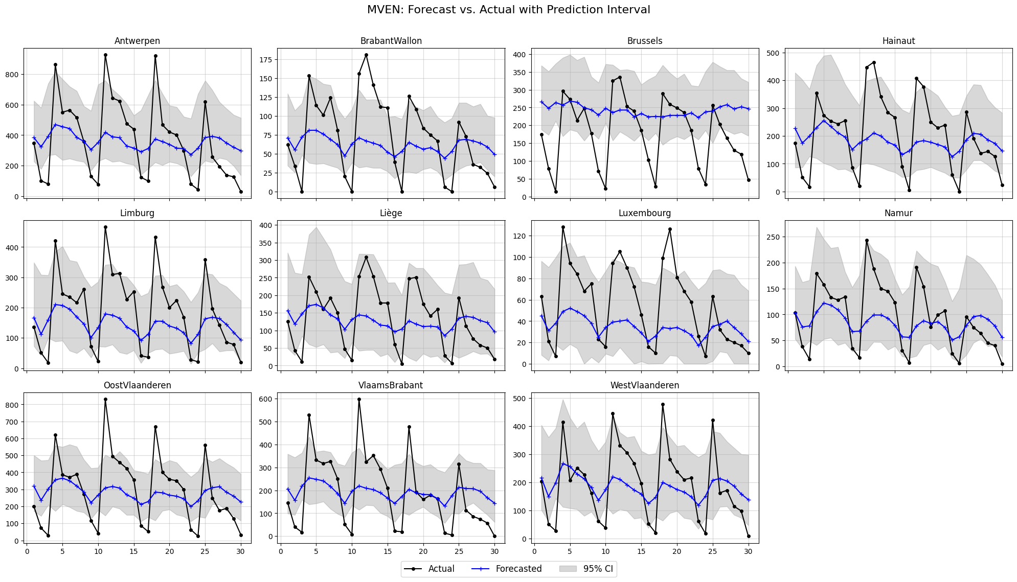
forecast_ensemble = mven.predict(test_history, m_samples = 100, unstandardize=[mean, std], device=device)
plot_forecasts(NUM_NODES, plots_per_row=4, t_pred=30, forecast_ensemble=forecast_ensemble, 
               ground_truth=test_ground_truth, confidence_level=0.95, node_names=node_names,
                   title='MVEN: Forecast vs. Actual with Prediction Interval')

4. GCEN

4.1 Training the GCEN Model

gcen = GCEN(in_feat_dim=IN_FEAT_DIM,
    gcn_out_feat=6,
    lstm_hidden_dim=91,
    lstm_num_layers=5,
    lstm_dropout=0.30479293048737066,
    p_lag=P_LAG,
    t_pred=T_PRED,
    graph_info=graph_info,
    graph_conv_params=graph_conv_params,
    noise_encode="add",
    noise_dist="uniform",
    gcn_seed=21,
    temporal_seed=9
).to(device)
optimizer = optim.Adam(gcen.parameters(), lr=0.00426979947571805) 

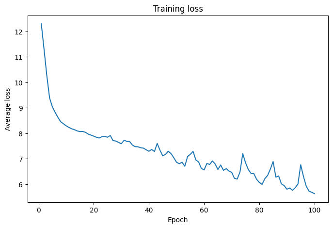
# Run Training
gcen.fit(data_loader=trainloader, optimizer=optimizer, loss_fn=energy_score_loss, num_epochs=100, m_samples=2, 
         device=device, monitor=True, visualize=True, verbose=False)

Training: 100%|██████████| 100/100 [01:03<00:00,  1.56epoch/s]

4.2 In-sample Diagnostics

# Getting the un-standardized in-sample predictions
in_sample_preds = gcen.predict_in_sample(train_tensor, m_samples = 100, method = "q_step", batch_size = 64, 
                                         device=device, unstandardize=[mean, std])

in_sample_preds.shape

torch.Size([100, 746, 11, 1])

# Evaluation of in-sample predictions
gcen.evaluate_in_sample_fit(train_tensor, m_samples = 100, n_repeats = 10,
        method = "q_step", batch_size = 64, point_method="median",
        unstandardize = [mean,std], device = device)

	SMAPE	MAE	RMSE	MASE	RMSSE	Pinball_80	Pinball_95	Rho-0.5	Rho-0.9	CRPS	EC	Winkler
mean	63.87	202.47	517.36	1.03	1.05	110.0	88.85	0.42	0.41	169.35	0.55	4072.27
std	0.12	0.68	3.54	0.00	0.01	0.5	0.74	0.00	0.00	0.50	0.00	46.93

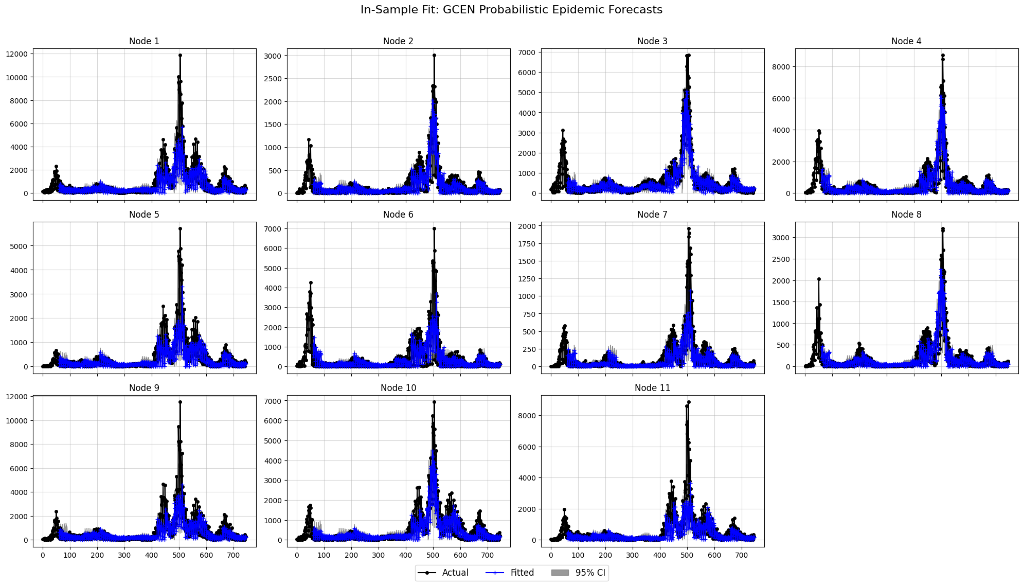
# Plotting the in-sample predictions vs training data and residuals
gcen.plot_in_sample_fit(
    in_sample_preds=in_sample_preds,
    original_data=y_train, # Ensure ground truth is also in original scale
    plots_per_row=4,
    confidence_level=0.95,
    title="In-Sample Fit: GCEN Probabilistic Epidemic Forecasts"
)

gcen.plot_residuals(
    residuals=residuals,
    plots_per_row=4,
    title="GCEN: Residuals (Actual - Predicted)"
)

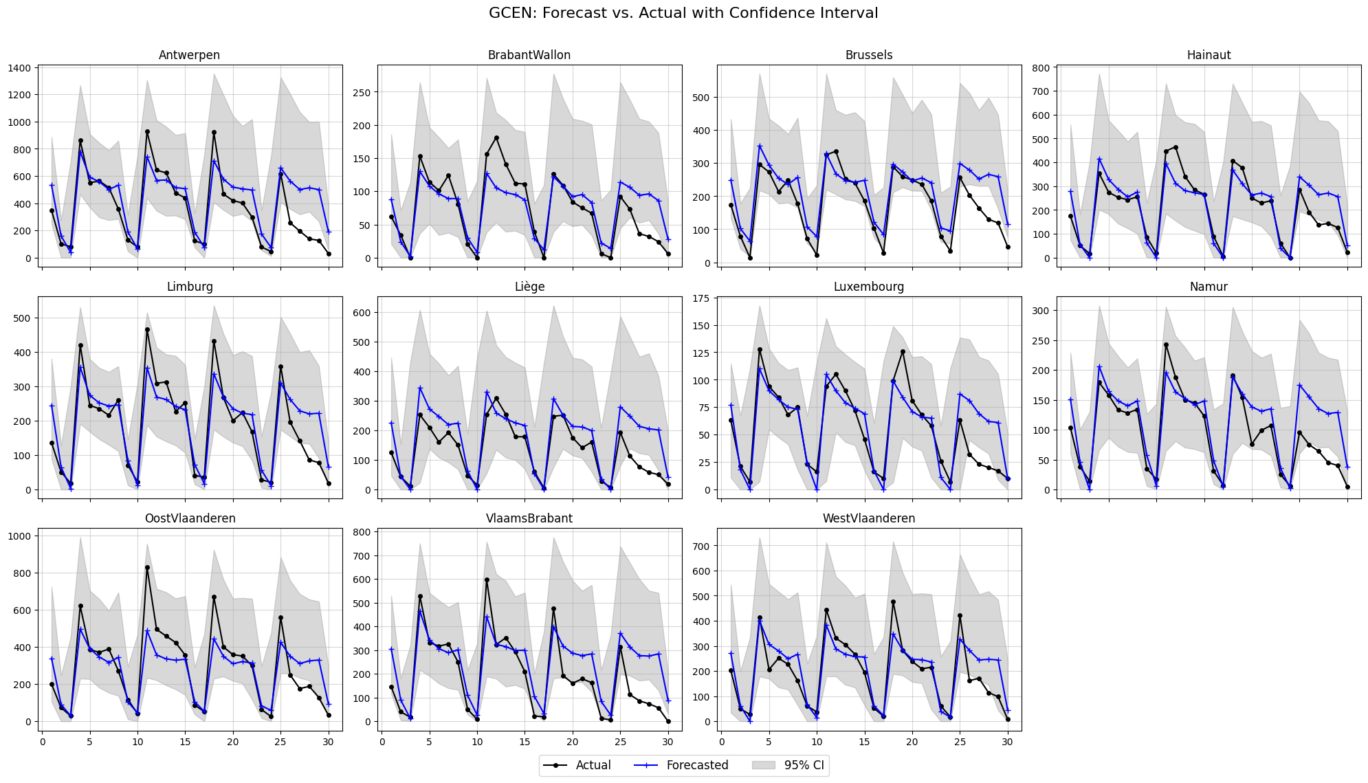
4.2 Out-of-sample Forecasts and Evaluation

metrics = gcen.evaluate_forecasts(m_samples=100, n_repeats=50, 
                              history=test_history, y_true=test_ground_truth, y_train=y_train, 
                              unstandardize=[mean, std])
display(metrics)

	SMAPE	MAE	RMSE	MASE	RMSSE	Pinball_80	Pinball_95	Rho-0.5	Rho-0.9	CRPS	EC	Winkler
mean	46.99	55.13	82.02	0.28	0.17	22.2	10.17	0.31	0.18	42.38	0.86	561.29
std	1.08	0.86	1.44	0.00	0.00	0.6	0.32	0.00	0.00	0.59	0.01	14.58

forecast_ensemble = gcen.predict(test_history, m_samples = 100, unstandardize=[mean, std], device=device)
plot_forecasts(NUM_NODES, plots_per_row=4, t_pred=30, forecast_ensemble=forecast_ensemble, 
               ground_truth=test_ground_truth, confidence_level=0.95, node_names=node_names,
                   title='GCEN: Forecast vs. Actual with Confidence Interval')

5. STEN

sten = STEN(in_feat_dim=IN_FEAT_DIM, embedding_dim=10, max_spatial_lag=max_spatial_lag, num_nodes=NUM_NODES, noise_dist="uniform",
           lstm_hidden_dim=39, lstm_num_layers=1, lstm_dropout=0.2433492165113465, 
           p_lag=P_LAG, t_pred=T_PRED, temporal_seed=9).to(device)

optimizer = optim.Adam(sten.parameters(), lr=0.0016437668357369587) 

# Run Training
sten.fit(data_loader=trainloader, optimizer=optimizer, loss_fn=energy_score_loss, num_epochs=100, m_samples=2, 
         device=device, monitor=True, visualize=True, verbose=False, W_list=W_list)

metrics = sten.evaluate(m_samples=100, n_repeats=50, 
                              history=test_history, y_true=test_ground_truth, y_train=y_train, 
                              unstandardize=[mean, std], W_list=W_list)
display(metrics)

Training: 100%|██████████| 100/100 [00:08<00:00, 11.42epoch/s]

	SMAPE	MAE	RMSE	MASE	RMSSE	Pinball_80	Pinball_95	Rho-0.5	Rho-0.9	CRPS	EC	Winkler
mean	68.29	100.76	136.04	0.51	0.28	38.57	21.37	0.57	0.33	79.06	0.53	1422.45
std	0.20	0.42	0.49	0.00	0.00	0.33	0.51	0.00	0.00	0.34	0.01	33.87

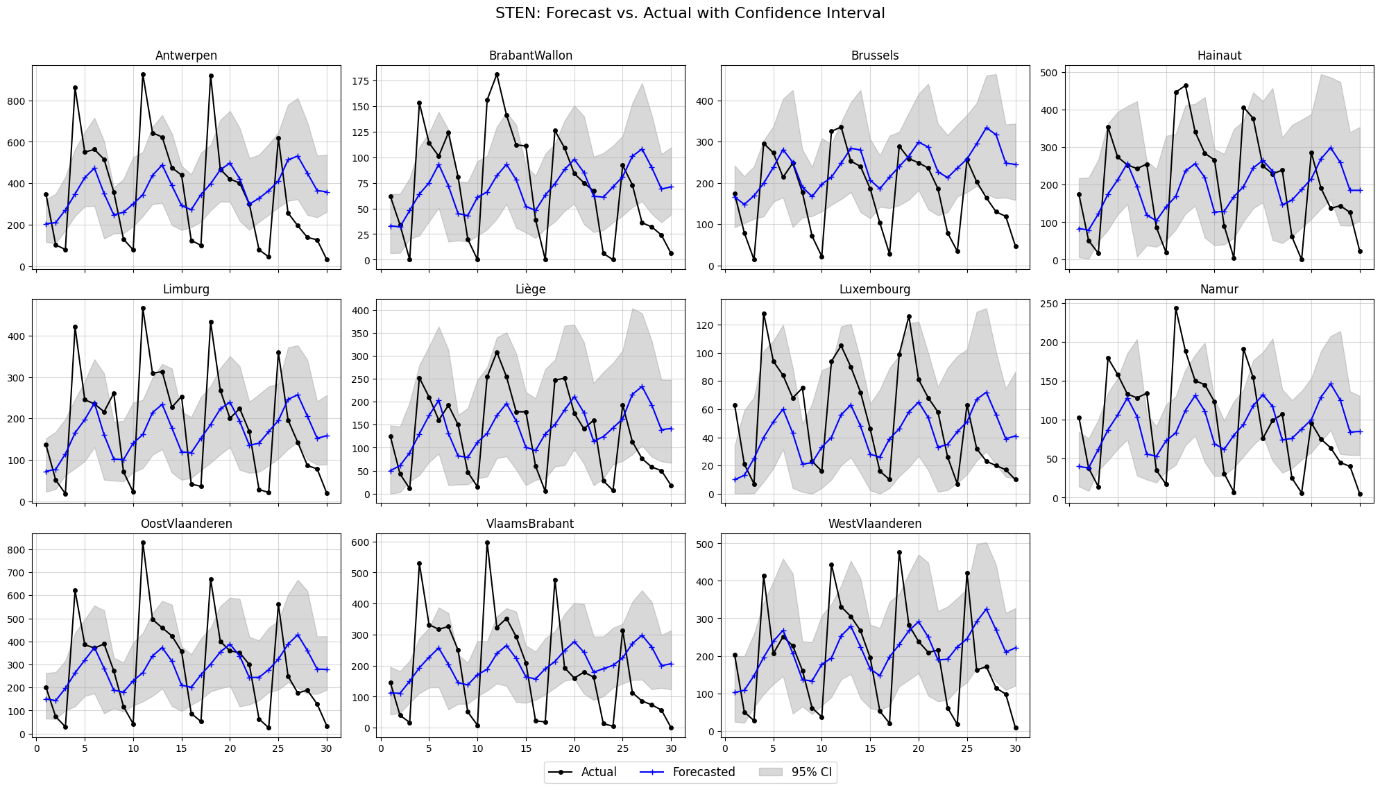
forecast_ensemble = sten.predict(test_history, m_samples = 100, unstandardize=[mean, std], device=device, W_list=W_list)
plot_forecasts(NUM_NODES, plots_per_row=4, t_pred=30, forecast_ensemble=forecast_ensemble, 
               ground_truth=test_ground_truth, confidence_level=0.95, node_names=node_names,
                   title='STEN: Forecast vs. Actual with Confidence Interval')